Single_Farm_Analysis_cowfootR

Comprehensive Single Farm Carbon Footprint Analysis

This vignette demonstrates how to conduct a detailed carbon footprint assessment for an individual dairy farm using all available functions in cowfootR. We’ll work through a realistic example with comprehensive data collection and analysis.

Farm Profile: Estancia Las Flores

For this analysis, we’ll assess a medium-sized dairy farm in Uruguay with the following characteristics:

Location: Temperate climate, well-drained soils
System: Mixed grazing with supplementation
Herd: 150 dairy cows plus young stock
Area: 200 hectares total
Production: 950,000 litres annually

Step 1: System Boundaries Definition

First, we define what emission sources to include in our assessment:

# Define comprehensive farm-gate boundaries
boundaries <- set_system_boundaries("farm_gate")
print(boundaries)
#> $scope
#> [1] "farm_gate"
#> 
#> $include
#> [1] "enteric" "manure"  "soil"    "energy"  "inputs"

# Alternative: cradle-to-farm-gate (includes upstream emissions)
boundaries_extended <- set_system_boundaries("cradle_to_farm_gate")
print(boundaries_extended)
#> $scope
#> [1] "cradle_to_farm_gate"
#> 
#> $include
#> [1] "feed"    "enteric" "manure"  "soil"    "energy"  "inputs"

# Custom boundaries example
boundaries_partial <- set_system_boundaries(
  scope = "partial",
  include = c("enteric", "manure", "soil")
)
print(boundaries_partial)
#> $scope
#> [1] "partial"
#> 
#> $include
#> [1] "enteric" "manure"  "soil"

For this analysis, we’ll use farm-gate boundaries as they represent the most common assessment scope.

Step 2: Detailed Farm Data Collection

Herd Composition and Management

# Detailed herd data
herd_data <- list(
  # Main herd
  dairy_cows_milking = 120,
  dairy_cows_dry = 30,
  
  # Young stock
  heifers_total = 45,
  calves_total = 35,
  bulls_total = 3,
  
  # Animal characteristics (kg live weight)
  body_weight_cows = 580,
  body_weight_heifers = 380,
  body_weight_calves = 180,
  body_weight_bulls = 750,
  
  # Production parameters
  milk_yield_per_cow = 6300,  # kg/cow/year
  annual_milk_litres = 950000,
  fat_percent = 3.7,
  protein_percent = 3.3,
  milk_density = 1.032
)

print(herd_data)
#> $dairy_cows_milking
#> [1] 120
#> 
#> $dairy_cows_dry
#> [1] 30
#> 
#> $heifers_total
#> [1] 45
#> 
#> $calves_total
#> [1] 35
#> 
#> $bulls_total
#> [1] 3
#> 
#> $body_weight_cows
#> [1] 580
#> 
#> $body_weight_heifers
#> [1] 380
#> 
#> $body_weight_calves
#> [1] 180
#> 
#> $body_weight_bulls
#> [1] 750
#> 
#> $milk_yield_per_cow
#> [1] 6300
#> 
#> $annual_milk_litres
#> [1] 950000
#> 
#> $fat_percent
#> [1] 3.7
#> 
#> $protein_percent
#> [1] 3.3
#> 
#> $milk_density
#> [1] 1.032

Feed and Nutrition Management

# Feed inputs (all in kg dry matter per year)
feed_data <- list(
  # Purchased feeds
  concentrate_kg = 220000,
  grain_dry_kg = 80000,
  grain_wet_kg = 45000,
  ration_kg = 60000,
  byproducts_kg = 25000,
  proteins_kg = 35000,
  
  # Nutritional parameters
  dry_matter_intake_cows = 19.5,  # kg DM/cow/day
  dry_matter_intake_heifers = 11.0,
  dry_matter_intake_calves = 6.0,
  dry_matter_intake_bulls = 14.0,
  ym_percent = 6.3  # Methane conversion factor
)

print(feed_data)
#> $concentrate_kg
#> [1] 220000
#> 
#> $grain_dry_kg
#> [1] 80000
#> 
#> $grain_wet_kg
#> [1] 45000
#> 
#> $ration_kg
#> [1] 60000
#> 
#> $byproducts_kg
#> [1] 25000
#> 
#> $proteins_kg
#> [1] 35000
#> 
#> $dry_matter_intake_cows
#> [1] 19.5
#> 
#> $dry_matter_intake_heifers
#> [1] 11
#> 
#> $dry_matter_intake_calves
#> [1] 6
#> 
#> $dry_matter_intake_bulls
#> [1] 14
#> 
#> $ym_percent
#> [1] 6.3

Land Use and Soil Management

# Detailed land use breakdown
land_data <- list(
  # Total areas (hectares)
  area_total = 200,
  area_productive = 185,
  area_fertilized = 160,
  
  # Area breakdown
  pasture_permanent = 140,
  pasture_temporary = 30,
  crops_feed = 12,
  crops_cash = 3,
  infrastructure = 8,
  woodland = 7,
  
  # Soil and climate
  soil_type = "well_drained",
  climate_zone = "temperate",
  
  # Nitrogen inputs (kg N/year)
  n_fertilizer_synthetic = 2400,
  n_fertilizer_organic = 500,
  n_excreta_pasture = 15000,  # Estimated from grazing
  n_crop_residues = 800
)

print(land_data)
#> $area_total
#> [1] 200
#> 
#> $area_productive
#> [1] 185
#> 
#> $area_fertilized
#> [1] 160
#> 
#> $pasture_permanent
#> [1] 140
#> 
#> $pasture_temporary
#> [1] 30
#> 
#> $crops_feed
#> [1] 12
#> 
#> $crops_cash
#> [1] 3
#> 
#> $infrastructure
#> [1] 8
#> 
#> $woodland
#> [1] 7
#> 
#> $soil_type
#> [1] "well_drained"
#> 
#> $climate_zone
#> [1] "temperate"
#> 
#> $n_fertilizer_synthetic
#> [1] 2400
#> 
#> $n_fertilizer_organic
#> [1] 500
#> 
#> $n_excreta_pasture
#> [1] 15000
#> 
#> $n_crop_residues
#> [1] 800

Energy Consumption

# Energy use breakdown
energy_data <- list(
  # Fuel consumption (litres/year)
  diesel_litres = 12000,
  petrol_litres = 1800,
  
  # Other energy sources
  lpg_kg = 600,
  natural_gas_m3 = 0,
  electricity_kwh = 48000,
  
  # Country for electricity factors
  country = "UY"
)

print(energy_data)
#> $diesel_litres
#> [1] 12000
#> 
#> $petrol_litres
#> [1] 1800
#> 
#> $lpg_kg
#> [1] 600
#> 
#> $natural_gas_m3
#> [1] 0
#> 
#> $electricity_kwh
#> [1] 48000
#> 
#> $country
#> [1] "UY"

Additional Inputs

# Other purchased inputs
other_inputs <- list(
  # Materials (kg/year)
  plastic_kg = 450,
  
  # Transport (optional)
  transport_km = 120,  # Average transport distance for feeds
  
  # Fertilizer types
  fert_type = "mixed",
  plastic_type = "mixed",
  
  # Regional factors
  region = "global"  # Can be "EU", "US", "Brazil", etc.
)

print(other_inputs)
#> $plastic_kg
#> [1] 450
#> 
#> $transport_km
#> [1] 120
#> 
#> $fert_type
#> [1] "mixed"
#> 
#> $plastic_type
#> [1] "mixed"
#> 
#> $region
#> [1] "global"

Step 3: Emission Calculations by Source

Now we calculate emissions from each source using the detailed farm data.

Enteric Fermentation Emissions

# Calculate enteric emissions for each animal category
enteric_cows <- calc_emissions_enteric(
  n_animals = herd_data$dairy_cows_milking + herd_data$dairy_cows_dry,
  cattle_category = "dairy_cows",
  avg_milk_yield = herd_data$milk_yield_per_cow,
  avg_body_weight = herd_data$body_weight_cows,
  dry_matter_intake = feed_data$dry_matter_intake_cows,
  ym_percent = feed_data$ym_percent,
  tier = 2,
  boundaries = boundaries
)

enteric_heifers <- calc_emissions_enteric(
  n_animals = herd_data$heifers_total,
  cattle_category = "heifers",
  avg_body_weight = herd_data$body_weight_heifers,
  dry_matter_intake = feed_data$dry_matter_intake_heifers,
  ym_percent = feed_data$ym_percent,
  tier = 2,
  boundaries = boundaries
)

enteric_calves <- calc_emissions_enteric(
  n_animals = herd_data$calves_total,
  cattle_category = "calves",
  avg_body_weight = herd_data$body_weight_calves,
  dry_matter_intake = feed_data$dry_matter_intake_calves,
  tier = 2,
  boundaries = boundaries
)

enteric_bulls <- calc_emissions_enteric(
  n_animals = herd_data$bulls_total,
  cattle_category = "bulls",
  avg_body_weight = herd_data$body_weight_bulls,
  dry_matter_intake = feed_data$dry_matter_intake_bulls,
  tier = 2,
  boundaries = boundaries
)

# Summary of enteric emissions
enteric_summary <- data.frame(
  Category = c("Dairy Cows", "Heifers", "Calves", "Bulls"),
  Animals = c(150, herd_data$heifers_total, herd_data$calves_total, herd_data$bulls_total),
  CH4_kg = c(enteric_cows$ch4_kg, enteric_heifers$ch4_kg, 
             enteric_calves$ch4_kg, enteric_bulls$ch4_kg),
  CO2eq_kg = c(enteric_cows$co2eq_kg, enteric_heifers$co2eq_kg,
               enteric_calves$co2eq_kg, enteric_bulls$co2eq_kg)
)

kable(enteric_summary, caption = "Enteric Emissions by Animal Category")

Enteric Emissions by Animal Category
Category	Animals	CH4_kg	CO2eq_kg
Dairy Cows	150	22299.26	606539.92
Heifers	45	3773.72	102645.22
Calves	35	1651.80	44928.88
Bulls	3	330.36	8985.78


# Total enteric emissions
total_enteric <- enteric_cows$co2eq_kg + enteric_heifers$co2eq_kg + 
                enteric_calves$co2eq_kg + enteric_bulls$co2eq_kg

Manure Management Emissions

# Calculate manure emissions for the entire herd
total_animals <- sum(herd_data$dairy_cows_milking, herd_data$dairy_cows_dry,
                    herd_data$heifers_total, herd_data$calves_total, herd_data$bulls_total)

manure_emissions <- calc_emissions_manure(
  n_cows = total_animals,
  manure_system = "pasture",  # Extensive grazing system
  tier = 2,
  avg_body_weight = 500,  # Weighted average
  diet_digestibility = 0.67,
  climate = "temperate",
  include_indirect = TRUE,
  boundaries = boundaries
)

print(manure_emissions)
#> $source
#> [1] "manure"
#> 
#> $system
#> [1] "pasture"
#> 
#> $tier
#> [1] 2
#> 
#> $climate
#> [1] "temperate"
#> 
#> $ch4_kg
#> [1] 4092.31
#> 
#> $n2o_direct_kg
#> [1] 732.29
#> 
#> $n2o_indirect_kg
#> [1] 134.56
#> 
#> $n2o_total_kg
#> [1] 866.84
#> 
#> $co2eq_kg
#> [1] 347959.2
#> 
#> $emission_factors
#> $emission_factors$ef_ch4
#> [1] NA
#> 
#> $emission_factors$ef_n2o_direct
#> [1] 0.02
#> 
#> $emission_factors$gwp_ch4
#> [1] 27.2
#> 
#> $emission_factors$gwp_n2o
#> [1] 273
#> 
#> 
#> $inputs
#> $inputs$n_cows
#> [1] 233
#> 
#> $inputs$n_excreted
#> [1] 100
#> 
#> $inputs$manure_system
#> [1] "pasture"
#> 
#> $inputs$include_indirect
#> [1] TRUE
#> 
#> $inputs$avg_body_weight
#> [1] 500
#> 
#> $inputs$diet_digestibility
#> [1] 0.67
#> 
#> 
#> $methodology
#> [1] "IPCC Tier 2 (VS_B0_MCF calculation)"
#> 
#> $standards
#> [1] "IPCC 2019 Refinement, IDF 2022"
#> 
#> $date
#> [1] "2025-09-11"
#> 
#> $per_cow
#> $per_cow$ch4_kg
#> [1] 17.5636
#> 
#> $per_cow$n2o_kg
#> [1] 3.720357
#> 
#> $per_cow$co2eq_kg
#> [1] 1493.387
#> 
#> 
#> $tier2_details
#> $tier2_details$vs_kg_per_day
#> [1] 26.6
#> 
#> $tier2_details$b0_used
#> [1] 0.18
#> 
#> $tier2_details$mcf_used
#> [1] 1.5

Soil N2O Emissions

# Calculate soil emissions from all N sources
soil_emissions <- calc_emissions_soil(
  n_fertilizer_synthetic = land_data$n_fertilizer_synthetic,
  n_fertilizer_organic = land_data$n_fertilizer_organic,
  n_excreta_pasture = land_data$n_excreta_pasture,
  n_crop_residues = land_data$n_crop_residues,
  area_ha = land_data$area_total,
  soil_type = land_data$soil_type,
  climate = land_data$climate_zone,
  include_indirect = TRUE,
  boundaries = boundaries
)

print(soil_emissions)
#> $source
#> [1] "soil"
#> 
#> $soil_conditions
#> $soil_conditions$soil_type
#> [1] "well_drained"
#> 
#> $soil_conditions$climate
#> [1] "temperate"
#> 
#> 
#> $nitrogen_inputs
#> $nitrogen_inputs$synthetic_fertilizer_kg_n
#> [1] 2400
#> 
#> $nitrogen_inputs$organic_fertilizer_kg_n
#> [1] 500
#> 
#> $nitrogen_inputs$excreta_pasture_kg_n
#> [1] 15000
#> 
#> $nitrogen_inputs$crop_residues_kg_n
#> [1] 800
#> 
#> $nitrogen_inputs$total_kg_n
#> [1] 18700
#> 
#> 
#> $emissions_breakdown
#> $emissions_breakdown$direct_n2o_kg
#> [1] 293.857
#> 
#> $emissions_breakdown$indirect_volatilization_n2o_kg
#> [1] 52.486
#> 
#> $emissions_breakdown$indirect_leaching_n2o_kg
#> [1] 66.118
#> 
#> $emissions_breakdown$total_indirect_n2o_kg
#> [1] 118.604
#> 
#> $emissions_breakdown$total_n2o_kg
#> [1] 412.461
#> 
#> 
#> $co2eq_kg
#> [1] 112601.8
#> 
#> $emission_factors
#> $emission_factors$ef_direct
#> [1] 0.01
#> 
#> $emission_factors$ef_volatilization
#> [1] 0.01
#> 
#> $emission_factors$ef_leaching
#> [1] 0.0075
#> 
#> $emission_factors$gwp_n2o
#> [1] 273
#> 
#> $emission_factors$factors_source
#> [1] "IPCC-style defaults (temperate, well_drained)"
#> 
#> 
#> $methodology
#> [1] "Tier 1-style (direct + indirect)"
#> 
#> $standards
#> [1] "IPCC 2019 Refinement, IDF 2022"
#> 
#> $date
#> [1] "2025-09-11"
#> 
#> $per_hectare_metrics
#> $per_hectare_metrics$n_input_kg_per_ha
#> [1] 93.5
#> 
#> $per_hectare_metrics$n2o_kg_per_ha
#> [1] 2.062
#> 
#> $per_hectare_metrics$co2eq_kg_per_ha
#> [1] 563.01
#> 
#> $per_hectare_metrics$emission_intensity_kg_co2eq_per_kg_n
#> [1] 6.02
#> 
#> 
#> $source_contributions
#> $source_contributions$synthetic_fertilizer_pct
#> [1] 12.8
#> 
#> $source_contributions$organic_fertilizer_pct
#> [1] 2.7
#> 
#> $source_contributions$excreta_pasture_pct
#> [1] 80.2
#> 
#> $source_contributions$crop_residues_pct
#> [1] 4.3
#> 
#> $source_contributions$direct_emissions_pct
#> [1] 71.2
#> 
#> $source_contributions$indirect_emissions_pct
#> [1] 28.8

# Calculate emissions from energy use
energy_emissions <- calc_emissions_energy(
  diesel_l = energy_data$diesel_litres,
  petrol_l = energy_data$petrol_litres,
  lpg_kg = energy_data$lpg_kg,
  natural_gas_m3 = energy_data$natural_gas_m3,
  electricity_kwh = energy_data$electricity_kwh,
  country = energy_data$country,
  include_upstream = FALSE,  # Only direct emissions
  boundaries = boundaries
)

print(energy_emissions)
#> $source
#> [1] "energy"
#> 
#> $fuel_emissions
#> $fuel_emissions$diesel_co2_kg
#> [1] 32040
#> 
#> $fuel_emissions$petrol_co2_kg
#> [1] 4158
#> 
#> $fuel_emissions$lpg_co2_kg
#> [1] 1800
#> 
#> $fuel_emissions$natural_gas_co2_kg
#> [1] 0
#> 
#> $fuel_emissions$electricity_co2_kg
#> [1] 3840
#> 
#> 
#> $direct_co2eq_kg
#> [1] 41838
#> 
#> $upstream_co2eq_kg
#> [1] 0
#> 
#> $co2eq_kg
#> [1] 41838
#> 
#> $emission_factors
#> $emission_factors$diesel_kg_co2_per_l
#> [1] 2.67
#> 
#> $emission_factors$petrol_kg_co2_per_l
#> [1] 2.31
#> 
#> $emission_factors$lpg_kg_co2_per_kg
#> [1] 3
#> 
#> $emission_factors$natural_gas_kg_co2_per_m3
#> [1] 2
#> 
#> $emission_factors$electricity_kg_co2_per_kwh
#> [1] 0.08
#> 
#> $emission_factors$electricity_country
#> [1] "UY"
#> 
#> 
#> $inputs
#> $inputs$diesel_l
#> [1] 12000
#> 
#> $inputs$petrol_l
#> [1] 1800
#> 
#> $inputs$lpg_kg
#> [1] 600
#> 
#> $inputs$natural_gas_m3
#> [1] 0
#> 
#> $inputs$electricity_kwh
#> [1] 48000
#> 
#> $inputs$include_upstream
#> [1] FALSE
#> 
#> 
#> $methodology
#> [1] "IPCC 2019 emission factors"
#> 
#> $standards
#> [1] "IPCC 2019 Refinement, IDF 2022"
#> 
#> $date
#> [1] "2025-09-11"
#> 
#> $energy_metrics
#> $energy_metrics$electricity_share_pct
#> [1] 9.2
#> 
#> $energy_metrics$fossil_fuel_share_pct
#> [1] 90.8
#> 
#> $energy_metrics$co2_intensity_kg_per_mwh
#> [1] 80

Purchased Input Emissions

# Calculate emissions from purchased inputs
input_emissions <- calc_emissions_inputs(
  conc_kg = feed_data$concentrate_kg,
  fert_n_kg = land_data$n_fertilizer_synthetic,
  plastic_kg = other_inputs$plastic_kg,
  feed_grain_dry_kg = feed_data$grain_dry_kg,
  feed_grain_wet_kg = feed_data$grain_wet_kg,
  feed_ration_kg = feed_data$ration_kg,
  feed_byproducts_kg = feed_data$byproducts_kg,
  feed_proteins_kg = feed_data$proteins_kg,
  region = other_inputs$region,
  fert_type = other_inputs$fert_type,
  plastic_type = other_inputs$plastic_type,
  transport_km = other_inputs$transport_km,
  boundaries = boundaries
)

print(input_emissions)
#> $source
#> [1] "inputs"
#> 
#> $emissions_breakdown
#> $emissions_breakdown$concentrate_co2eq_kg
#> [1] 154000
#> 
#> $emissions_breakdown$fertilizer_co2eq_kg
#> [1] 15840
#> 
#> $emissions_breakdown$plastic_co2eq_kg
#> [1] 1125
#> 
#> $emissions_breakdown$feeds_co2eq_kg
#>  grain_dry  grain_wet     ration byproducts   proteins       corn        soy 
#>      32000      13500      36000       3750      63000          0          0 
#>      wheat 
#>          0 
#> 
#> $emissions_breakdown$total_feeds_co2eq_kg
#> [1] 148250
#> 
#> $emissions_breakdown$transport_adjustment_co2eq_kg
#> [1] 5580
#> 
#> 
#> $co2eq_kg
#> [1] 324795
#> 
#> $total_co2eq_kg
#> [1] 324795
#> 
#> $region
#> [1] "global"
#> 
#> $emission_factors_used
#> $emission_factors_used$concentrate
#> $emission_factors_used$concentrate$value
#> [1] 0.7
#> 
#> $emission_factors_used$concentrate$unit
#> [1] "kg CO2e/kg"
#> 
#> 
#> $emission_factors_used$fertilizer
#> $emission_factors_used$fertilizer$value
#> [1] 6.6
#> 
#> $emission_factors_used$fertilizer$type
#> [1] "mixed"
#> 
#> $emission_factors_used$fertilizer$unit
#> [1] "kg CO2e/kg N"
#> 
#> 
#> $emission_factors_used$plastic
#> $emission_factors_used$plastic$value
#> [1] 2.5
#> 
#> $emission_factors_used$plastic$type
#> [1] "mixed"
#> 
#> $emission_factors_used$plastic$unit
#> [1] "kg CO2e/kg"
#> 
#> 
#> $emission_factors_used$feeds
#> $emission_factors_used$feeds$grain_dry
#> $emission_factors_used$feeds$grain_dry$value
#> [1] 0.4
#> 
#> $emission_factors_used$feeds$grain_dry$unit
#> [1] "kg CO2e/kg"
#> 
#> 
#> $emission_factors_used$feeds$grain_wet
#> $emission_factors_used$feeds$grain_wet$value
#> [1] 0.3
#> 
#> $emission_factors_used$feeds$grain_wet$unit
#> [1] "kg CO2e/kg"
#> 
#> 
#> $emission_factors_used$feeds$ration
#> $emission_factors_used$feeds$ration$value
#> [1] 0.6
#> 
#> $emission_factors_used$feeds$ration$unit
#> [1] "kg CO2e/kg"
#> 
#> 
#> $emission_factors_used$feeds$byproducts
#> $emission_factors_used$feeds$byproducts$value
#> [1] 0.15
#> 
#> $emission_factors_used$feeds$byproducts$unit
#> [1] "kg CO2e/kg"
#> 
#> 
#> $emission_factors_used$feeds$proteins
#> $emission_factors_used$feeds$proteins$value
#> [1] 1.8
#> 
#> $emission_factors_used$feeds$proteins$unit
#> [1] "kg CO2e/kg"
#> 
#> 
#> $emission_factors_used$feeds$corn
#> $emission_factors_used$feeds$corn$value
#> [1] 0.45
#> 
#> $emission_factors_used$feeds$corn$unit
#> [1] "kg CO2e/kg"
#> 
#> 
#> $emission_factors_used$feeds$soy
#> $emission_factors_used$feeds$soy$value
#> [1] 2.1
#> 
#> $emission_factors_used$feeds$soy$unit
#> [1] "kg CO2e/kg"
#> 
#> 
#> $emission_factors_used$feeds$wheat
#> $emission_factors_used$feeds$wheat$value
#> [1] 0.52
#> 
#> $emission_factors_used$feeds$wheat$unit
#> [1] "kg CO2e/kg"
#> 
#> 
#> 
#> $emission_factors_used$region_source
#> [1] "global"
#> 
#> $emission_factors_used$transport_km
#> [1] 120
#> 
#> 
#> $inputs_summary
#> $inputs_summary$concentrate_kg
#> [1] 220000
#> 
#> $inputs_summary$fertilizer_n_kg
#> [1] 2400
#> 
#> $inputs_summary$plastic_kg
#> [1] 450
#> 
#> $inputs_summary$total_feeds_kg
#> [1] 245000
#> 
#> $inputs_summary$feed_breakdown_kg
#> $inputs_summary$feed_breakdown_kg$grain_dry
#> [1] 80000
#> 
#> $inputs_summary$feed_breakdown_kg$grain_wet
#> [1] 45000
#> 
#> $inputs_summary$feed_breakdown_kg$ration
#> [1] 60000
#> 
#> $inputs_summary$feed_breakdown_kg$byproducts
#> [1] 25000
#> 
#> $inputs_summary$feed_breakdown_kg$proteins
#> [1] 35000
#> 
#> $inputs_summary$feed_breakdown_kg$corn
#> [1] 0
#> 
#> $inputs_summary$feed_breakdown_kg$soy
#> [1] 0
#> 
#> $inputs_summary$feed_breakdown_kg$wheat
#> [1] 0
#> 
#> 
#> 
#> $contribution_analysis
#> $contribution_analysis$concentrate_pct
#> [1] 47.4
#> 
#> $contribution_analysis$fertilizer_pct
#> [1] 4.9
#> 
#> $contribution_analysis$plastic_pct
#> [1] 0.3
#> 
#> $contribution_analysis$feeds_pct
#> [1] 45.6
#> 
#> $contribution_analysis$transport_pct
#> [1] 1.7
#> 
#> 
#> $uncertainty
#> NULL
#> 
#> $methodology
#> [1] "Regional emission factors with optional uncertainty analysis"
#> 
#> $standards
#> [1] "IDF 2022; generic LCI sources"
#> 
#> $date
#> [1] "2025-09-11"

Step 4: Total Emissions and Analysis

Aggregate All Emission Sources

# Create combined enteric emissions object
enteric_combined <- list(
  source = "enteric",
  co2eq_kg = total_enteric
)

# Calculate total emissions
total_emissions <- calc_total_emissions(
  enteric_combined,
  manure_emissions,
  soil_emissions,
  energy_emissions,
  input_emissions
)

total_emissions
#> Carbon Footprint - Total Emissions
#> ==================================
#> Total CO2eq: 1590294 kg
#> Number of sources: 5 
#> 
#> Breakdown by source:
#>   energy : 41838 kg CO2eq
#>   enteric : 763099.8 kg CO2eq
#>   inputs : 324795 kg CO2eq
#>   manure : 347959.2 kg CO2eq
#>   soil : 112601.8 kg CO2eq
#> 
#> Calculated on: 2025-09-11

Visualize Emission Sources

# Create detailed breakdown
emission_breakdown <- data.frame(
  Source = names(total_emissions$breakdown),
  Emissions = as.numeric(total_emissions$breakdown),
  Percentage = round(as.numeric(total_emissions$breakdown) / 
                    total_emissions$total_co2eq * 100, 1)
)

# Create bar chart
ggplot(emission_breakdown, aes(x = reorder(Source, Emissions), y = Emissions)) +
  geom_col(fill = "steelblue", alpha = 0.8) +
  geom_text(aes(label = paste0(Percentage, "%")), 
            hjust = -0.1, size = 3) +
  coord_flip() +
  labs(title = "Farm Emissions by Source",
       subtitle = paste("Total:", format(round(total_emissions$total_co2eq), 
                         big.mark = ","), "kg CO₂eq/year"),
       x = "Emission Source",
       y = "Emissions (kg CO₂eq/year)") +
  theme_minimal() +
  theme(plot.title = element_text(size = 14, hjust = 0.5),
        plot.subtitle = element_text(hjust = 0.5))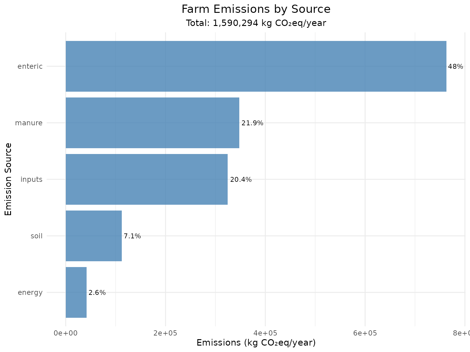

Figura generada por la viñeta; ver texto para detalles.

Step 5: Intensity Calculations

Milk Intensity

# Calculate emissions per kg of FPCM
milk_intensity <- calc_intensity_litre(
  total_emissions = total_emissions,
  milk_litres = herd_data$annual_milk_litres,
  fat = herd_data$fat_percent,
  protein = herd_data$protein_percent,
  milk_density = herd_data$milk_density
)

print(milk_intensity)
#> Carbon Footprint Intensity
#> ==========================
#> Intensity: 1.684 kg CO2eq/kg FPCM
#> 
#> Production data:
#>  Raw milk (L): 950,000 L
#>  Raw milk (kg): 980,400 kg
#>  FPCM (kg): 944,223 kg
#>  Fat content: 3.7 %
#>  Protein content: 3.3 %
#> 
#> Total emissions: 1,590,294 kg CO2eq
#> Calculated on: 2025-09-11

Area Intensity

# Calculate emissions per hectare
area_breakdown <- list(
  pasture_permanent = land_data$pasture_permanent,
  pasture_temporary = land_data$pasture_temporary,
  crops_feed = land_data$crops_feed,
  crops_cash = land_data$crops_cash,
  infrastructure = land_data$infrastructure,
  woodland = land_data$woodland
)

area_intensity <- calc_intensity_area(
  total_emissions = total_emissions,
  area_total_ha = land_data$area_total,
  area_productive_ha = land_data$area_productive,
  area_breakdown = area_breakdown,
  validate_area_sum = TRUE
)

print(area_intensity)
#> Carbon Footprint Area Intensity
#> ===============================
#> Intensity (total area): 7951.47 kg CO2eq/ha
#> Intensity (productive area): 8596.18 kg CO2eq/ha
#> 
#> Area summary:
#>  Total area: 200 ha
#>  Productive area: 185 ha
#>  Land use efficiency: 92.5%
#> 
#> Land use breakdown:
#>  pasture permanent: 140.0 ha (70.0%) -> 1113206 kg CO2eq
#>  pasture temporary: 30.0 ha (15.0%) -> 238544 kg CO2eq
#>  crops feed: 12.0 ha (6.0%) -> 95418 kg CO2eq
#>  crops cash: 3.0 ha (1.5%) -> 23854 kg CO2eq
#>  infrastructure: 8.0 ha (4.0%) -> 63612 kg CO2eq
#>  woodland: 7.0 ha (3.5%) -> 55660 kg CO2eq
#> 
#> Total emissions: 1,590,294 kg CO2eq
#> Calculated on: 2025-09-11

Benchmarking Against Regional Standards

# Benchmark against Uruguayan standards
area_benchmark <- benchmark_area_intensity(
  cf_area_intensity = area_intensity,
  region = "uruguay"
)

print(area_benchmark$benchmarking)
#> $region
#> [1] "uruguay"
#> 
#> $benchmark_mean
#> [1] 6000
#> 
#> $benchmark_range
#> [1] 5000 7000
#> 
#> $benchmark_source
#> [1] "Placeholder"
#> 
#> $vs_mean_percent
#> [1] 43.3
#> 
#> $performance_category
#> [1] "Above average (above typical range)"

Step 6: Detailed Results Analysis

Per-Animal Emissions

# Calculate emissions per animal category
per_animal_analysis <- data.frame(
  Category = c("Dairy Cows", "All Animals"),
  Number = c(150, total_animals),
  Total_Emissions = c(total_emissions$total_co2eq, total_emissions$total_co2eq),
  Emissions_per_Head = c(
    total_emissions$total_co2eq / 150,
    total_emissions$total_co2eq / total_animals
  ),
  Milk_per_Head = c(herd_data$annual_milk_litres / 150, NA)
)

kable(per_animal_analysis, 
      digits = 0,
      caption = "Per-Animal Emission Analysis")

Per-Animal Emission Analysis
Category	Number	Total_Emissions	Emissions_per_Head	Milk_per_Head
Dairy Cows	150	1590294	10602	6333
All Animals	233	1590294	6825	NA

Feed Efficiency Analysis

# Calculate feed-related metrics
total_purchased_feed <- sum(
  feed_data$concentrate_kg,
  feed_data$grain_dry_kg,
  feed_data$grain_wet_kg,
  feed_data$ration_kg,
  feed_data$byproducts_kg,
  feed_data$proteins_kg
)

feed_analysis <- data.frame(
  Metric = c("Total Feed Purchases", "Feed Emissions", "Feed CO2eq per kg DM",
             "Feed Efficiency", "Milk from Feed"),
  Value = c(
    total_purchased_feed,
    input_emissions$total_co2eq_kg,
    input_emissions$total_co2eq_kg / total_purchased_feed,
    herd_data$annual_milk_litres / total_purchased_feed,
    herd_data$annual_milk_litres
  ),
  Unit = c("kg DM", "kg CO₂eq", "kg CO₂eq/kg DM", "L milk/kg DM", "L")
)

kable(feed_analysis, digits = 2, caption = "Feed Efficiency Analysis")

Feed Efficiency Analysis
Metric	Value	Unit
Total Feed Purchases	465000.00	kg DM
Feed Emissions	324795.00	kg CO₂eq
Feed CO2eq per kg DM	0.70	kg CO₂eq/kg DM
Feed Efficiency	2.04	L milk/kg DM
Milk from Feed	950000.00	L

Step 7: Mitigation Scenario Analysis

Let’s analyze potential mitigation strategies:

Scenario 1: Improved Feed Efficiency

# Scenario: 10% reduction in concentrate use with maintained production
improved_inputs <- calc_emissions_inputs(
  conc_kg = feed_data$concentrate_kg * 0.9,  # 10% reduction
  fert_n_kg = land_data$n_fertilizer_synthetic,
  plastic_kg = other_inputs$plastic_kg,
  feed_grain_dry_kg = feed_data$grain_dry_kg,
  feed_grain_wet_kg = feed_data$grain_wet_kg,
  feed_ration_kg = feed_data$ration_kg,
  feed_byproducts_kg = feed_data$byproducts_kg,
  feed_proteins_kg = feed_data$proteins_kg,
  region = other_inputs$region,
  fert_type = other_inputs$fert_type,
  plastic_type = other_inputs$plastic_type,
  transport_km = other_inputs$transport_km,
  boundaries = boundaries
)

# Calculate total for improved scenario
total_improved <- calc_total_emissions(
  enteric_combined,
  manure_emissions,
  soil_emissions,
  energy_emissions,
  improved_inputs
)

# Compare scenarios
scenario_comparison <- data.frame(
  Scenario = c("Baseline", "Improved Feed Efficiency"),
  Total_Emissions = c(total_emissions$total_co2eq, total_improved$total_co2eq),
  Input_Emissions = c(input_emissions$total_co2eq_kg, improved_inputs$total_co2eq_kg),
  Reduction_kg = c(0, total_emissions$total_co2eq - total_improved$total_co2eq),
  Reduction_percent = c(0, round((total_emissions$total_co2eq - total_improved$total_co2eq) / 
                               total_emissions$total_co2eq * 100, 1))
)

kable(scenario_comparison, caption = "Mitigation Scenario Analysis")

Mitigation Scenario Analysis
Scenario	Total_Emissions	Input_Emissions	Reduction_kg	Reduction_percent
Baseline	1590294	324795	0	0
Improved Feed Efficiency	1574630	309131	15664	1

Scenario 2: Enhanced Manure Management

# Scenario: Switch from pasture to anaerobic digester
improved_manure <- calc_emissions_manure(
  n_cows = total_animals,
  manure_system = "anaerobic_digester",
  tier = 2,
  avg_body_weight = 500,
  diet_digestibility = 0.67,
  climate = "temperate",
  retention_days = 45,
  system_temperature = 35,
  include_indirect = TRUE,
  boundaries = boundaries
)

# Calculate total with improved manure management
total_improved_manure <- calc_total_emissions(
  enteric_combined,
  improved_manure,
  soil_emissions,
  energy_emissions,
  input_emissions
)

manure_comparison <- data.frame(
  System = c("Pasture", "Anaerobic Digester"),
  CH4_kg = c(manure_emissions$ch4_kg, improved_manure$ch4_kg),
  N2O_kg = c(manure_emissions$n2o_total_kg, improved_manure$n2o_total_kg),
  Total_CO2eq = c(manure_emissions$co2eq_kg, improved_manure$co2eq_kg),
  Reduction_kg = c(0, manure_emissions$co2eq_kg - improved_manure$co2eq_kg)
)

kable(manure_comparison, caption = "Manure Management Comparison")

Manure Management Comparison
System	CH4_kg	N2O_kg	Total_CO2eq	Reduction_kg
Pasture	4092.31	866.84	347959.2	0
Anaerobic Digester	245538.86	866.84	6915305.2	-6567346

Step 8: Comprehensive Results Visualization

Multi-Source Emissions Chart

# Prepare data for comprehensive visualization
detailed_emissions <- data.frame(
  Source = c("Enteric - Cows", "Enteric - Young Stock", "Manure Management",
             "Soil N2O", "Energy Use", "Purchased Inputs"),
  Emissions = c(
    enteric_cows$co2eq_kg,
    enteric_heifers$co2eq_kg + enteric_calves$co2eq_kg + enteric_bulls$co2eq_kg,
    manure_emissions$co2eq_kg,
    soil_emissions$co2eq_kg,
    energy_emissions$co2eq_kg,
    input_emissions$total_co2eq_kg
  ),
  Category = c("Enteric", "Enteric", "Manure", "Soil", "Energy", "Inputs")
)

# Create stacked bar chart
ggplot(detailed_emissions, aes(x = "Farm Emissions", y = Emissions, fill = Source)) +
  geom_col() +
  geom_text(aes(label = ifelse(Emissions > 2000, 
                              paste0(round(Emissions/1000, 1), "k"), "")),
            position = position_stack(vjust = 0.5),
            color = "white", fontweight = "bold") +
  labs(title = "Estancia Las Flores - Carbon Footprint Breakdown",
       subtitle = paste("Total:", format(round(total_emissions$total_co2eq), 
                       big.mark = ","), "kg CO₂eq/year"),
       x = "",
       y = "Emissions (kg CO₂eq/year)") +
  theme_minimal() +
  theme(plot.title = element_text(size = 14, hjust = 0.5),
        plot.subtitle = element_text(hjust = 0.5),
        axis.text.x = element_blank(),
        legend.position = "right") +
  scale_fill_brewer(type = "qual", palette = "Set2")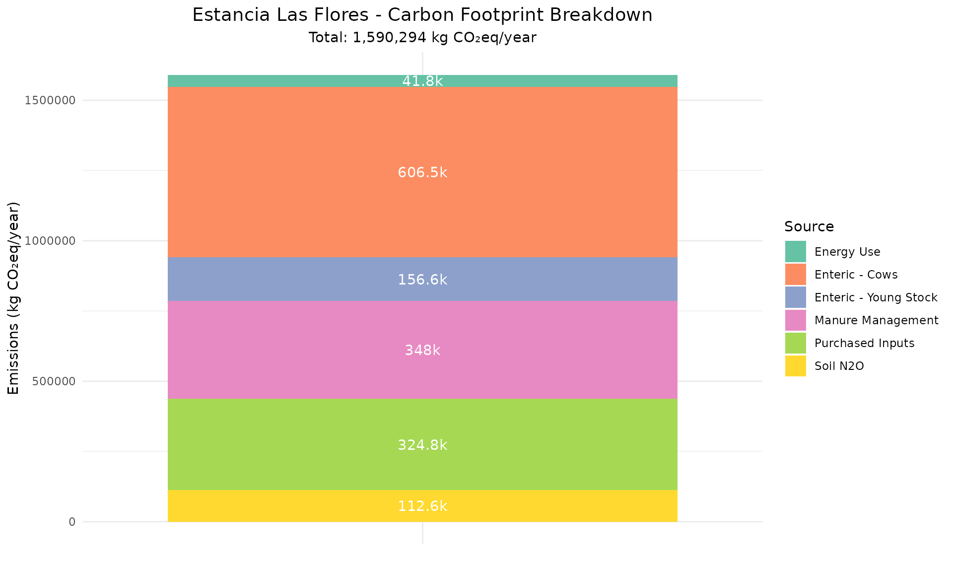

Figura generada por la viñeta; ver texto para detalles.

Intensity Metrics Dashboard

# Calculate key performance indicators
kpi_summary <- data.frame(
  Metric = c(
    "Milk Intensity (kg CO₂eq/kg FPCM)",
    "Area Intensity - Total (kg CO₂eq/ha)",
    "Area Intensity - Productive (kg CO₂eq/ha)",
    "Land Use Efficiency (%)",
    "Milk Yield (L/cow/year)",
    "Stocking Rate (cows/ha)"
  ),
  Value = c(
    round(milk_intensity$intensity_co2eq_per_kg_fpcm, 3),
    round(area_intensity$intensity_per_total_ha, 0),
    round(area_intensity$intensity_per_productive_ha, 0),
    round(area_intensity$land_use_efficiency * 100, 1),
    round(herd_data$annual_milk_litres / 150, 0),
    round(150 / land_data$area_total, 2)
  ),
  Benchmark = c("< 1.2", "< 8,000", "< 8,500", "> 85%", "> 6,000", "0.5-1.2"),
  Performance = c(
    ifelse(milk_intensity$intensity_co2eq_per_kg_fpcm < 1.2, "Good", "Needs Improvement"),
    ifelse(area_intensity$intensity_per_total_ha < 8000, "Good", "Needs Improvement"),
    ifelse(area_intensity$intensity_per_productive_ha < 8500, "Good", "Needs Improvement"),
    ifelse(area_intensity$land_use_efficiency > 0.85, "Good", "Needs Improvement"),
    ifelse(herd_data$annual_milk_litres / 150 > 6000, "Good", "Needs Improvement"),
    "Within Range"
  )
)

kable(kpi_summary, caption = "Key Performance Indicators")

Key Performance Indicators
Metric	Value	Benchmark	Performance
Milk Intensity (kg CO₂eq/kg FPCM)	1.684	< 1.2	Needs Improvement
Area Intensity - Total (kg CO₂eq/ha)	7951.000	< 8,000	Good
Area Intensity - Productive (kg CO₂eq/ha)	8596.000	< 8,500	Needs Improvement
Land Use Efficiency (%)	92.500	> 85%	Good
Milk Yield (L/cow/year)	6333.000	> 6,000	Good
Stocking Rate (cows/ha)	0.750	0.5-1.2	Within Range

Conclusion

This detailed single-farm analysis demonstrates the comprehensive capabilities of cowfootR for dairy farm carbon footprint assessment. The modular approach allows for detailed investigation of each emission source while maintaining consistency with international standards.

Key takeaways from this analysis:

Systematic approach: Following the step-by-step methodology ensures completeness and accuracy
Data quality matters: More detailed farm-specific data leads to more accurate results
Benchmarking provides context: Comparing results against regional standards helps identify improvement opportunities
Scenario analysis: Testing mitigation strategies helps prioritize actions
Uncertainty awareness: Understanding data limitations guides decision-making

For processing multiple farms simultaneously, see the “Batch Farm Assessment” vignette. For methodology details, consult the “IPCC Tier Comparison” vignette.

This analysis used cowfootR version 0.1.1 following IDF 2022 and IPCC 2019 standards.

Comprehensive Single Farm Carbon Footprint Analysis

Farm Profile: Estancia Las Flores

Step 1: System Boundaries Definition

Step 2: Detailed Farm Data Collection

Herd Composition and Management

Feed and Nutrition Management

Land Use and Soil Management

Energy Consumption

Additional Inputs

Step 3: Emission Calculations by Source

Enteric Fermentation Emissions

Manure Management Emissions

Soil N2O Emissions

Energy-Related Emissions

Purchased Input Emissions

Step 4: Total Emissions and Analysis

Aggregate All Emission Sources

Visualize Emission Sources

Step 5: Intensity Calculations

Milk Intensity

Area Intensity

Benchmarking Against Regional Standards

Step 6: Detailed Results Analysis

Per-Animal Emissions

Feed Efficiency Analysis

Step 7: Mitigation Scenario Analysis

Scenario 1: Improved Feed Efficiency

Scenario 2: Enhanced Manure Management

Step 8: Comprehensive Results Visualization

Multi-Source Emissions Chart

Intensity Metrics Dashboard

Conclusion