IPCC_Methodology_Tiers_cowfootR • cowfootR

Understanding IPCC Methodology Tiers

The Intergovernmental Panel on Climate Change (IPCC) provides three tiers of methodological complexity for greenhouse gas inventory calculations. cowfootR implements Tier 1 and Tier 2 methodologies for dairy farm carbon footprint assessments. This vignette explains the differences, when to use each approach, and demonstrates their practical application.

Theoretical Background

IPCC Tier System Overview

The IPCC tier system balances accuracy with data requirements and complexity:

Tier 1: Default emission factors with basic activity data
Tier 2: Country/region-specific factors with detailed activity data
Tier 3: Advanced modeling with comprehensive measurements (not implemented in cowfootR)

Key Differences in Dairy Applications

Aspect	Tier 1	Tier 2
Emission Factors	IPCC default values	Region/farm-specific values
Data Requirements	Basic (animal numbers, production)	Detailed (weights, intake, composition)
Accuracy	±25-50%	±10-25%
Time Investment	Low (hours)	Medium (days)
Suitable For	Screening, regional estimates	Farm management, policy

Methodological Differences by Emission Source

Enteric Fermentation

Tier 1 Approach

Uses fixed emission factors by animal category and production system
Based on broad regional averages
No consideration of diet quality or animal performance

# Tier 1 enteric calculation example
enteric_tier1 <- calc_emissions_enteric(
  n_animals = 100,
  cattle_category = "dairy_cows",
  production_system = "mixed",
  tier = 1  # Uses default emission factors
)

print(enteric_tier1$emission_factors)
#> $emission_factor_ch4
#> [1] 115
#> 
#> $ym_percent
#> [1] 6.5
#> 
#> $gwp_ch4
#> [1] 27.2
#> 
#> $method_used
#> [1] "Tier 1"

Tier 2 Approach

Calculates methane based on energy intake and conversion efficiency
Accounts for diet digestibility, animal productivity, and body weight
Uses farm-specific or regional Ym (methane conversion) factors

# Tier 2 enteric calculation with detailed parameters
enteric_tier2 <- calc_emissions_enteric(
  n_animals = 100,
  cattle_category = "dairy_cows",
  avg_milk_yield = 7200,
  avg_body_weight = 580,
  dry_matter_intake = 19.5,
  ym_percent = 6.2,
  tier = 2  # Uses energy-based calculation
)

print(enteric_tier2$emission_factors)
#> $emission_factor_ch4
#> [1] 146.302
#> 
#> $ym_percent
#> [1] 6.2
#> 
#> $gwp_ch4
#> [1] 27.2
#> 
#> $method_used
#> [1] "Tier 2"

Manure Management

Tier 1 vs Tier 2 Comparison

# Tier 1: Simple emission factors
manure_tier1 <- calc_emissions_manure(
  n_cows = 100,
  manure_system = "liquid_storage",
  tier = 1
)

# Tier 2: VS and MCF-based calculation
manure_tier2 <- calc_emissions_manure(
  n_cows = 100,
  manure_system = "liquid_storage",
  tier = 2,
  avg_body_weight = 580,
  diet_digestibility = 0.68,
  climate = "temperate",
  retention_days = 90,
  system_temperature = 20
)

# Compare results
manure_comparison <- data.frame(
  Tier = c("Tier 1", "Tier 2"),
  CH4_kg = c(manure_tier1$ch4_kg, manure_tier2$ch4_kg),
  N2O_kg = c(manure_tier1$n2o_total_kg, manure_tier2$n2o_total_kg),
  CO2eq_kg = c(manure_tier1$co2eq_kg, manure_tier2$co2eq_kg),
  Method = c("Default factors", "VS + MCF calculation")
)

kable(manure_comparison, caption = "Manure Management: Tier 1 vs Tier 2")

Manure Management: Tier 1 vs Tier 2
Tier	CH4_kg	N2O_kg	CO2eq_kg	Method
Tier 1	3000.00	314.29	167400	Default factors
Tier 2	52573.48	314.29	1515799	VS + MCF calculation

Comprehensive Farm Comparison

Let’s compare both tiers using a realistic farm example:

Farm Profile

# Define comprehensive farm data
farm_profile <- list(
  # Basic data (required for both tiers)
  dairy_cows = 120,
  heifers = 35,
  calves = 40,
  milk_production = 850000,  # litres/year
  farm_area = 160,  # hectares
  
  # Detailed data (enhances Tier 2)
  cow_body_weight = 580,
  heifer_body_weight = 380,
  calf_body_weight = 170,
  milk_yield_per_cow = 7080,
  cow_dm_intake = 19.2,
  heifer_dm_intake = 11.5,
  calf_dm_intake = 6.2,
  diet_digestibility = 0.67,
  ym_factor = 6.1,
  
  # Management data
  concentrate_feed = 195000,  # kg/year
  n_fertilizer = 2200,  # kg N/year
  diesel_use = 9500,  # litres/year
  electricity = 52000  # kWh/year
)

print(farm_profile[1:8])
#> $dairy_cows
#> [1] 120
#> 
#> $heifers
#> [1] 35
#> 
#> $calves
#> [1] 40
#> 
#> $milk_production
#> [1] 850000
#> 
#> $farm_area
#> [1] 160
#> 
#> $cow_body_weight
#> [1] 580
#> 
#> $heifer_body_weight
#> [1] 380
#> 
#> $calf_body_weight
#> [1] 170

Tier 1 Assessment

# Complete Tier 1 assessment
boundaries <- set_system_boundaries("farm_gate")

# Tier 1 calculations
enteric_t1 <- calc_emissions_enteric(
  n_animals = farm_profile$dairy_cows,
  cattle_category = "dairy_cows",
  tier = 1,
  boundaries = boundaries
)

heifers_t1 <- calc_emissions_enteric(
  n_animals = farm_profile$heifers,
  cattle_category = "heifers", 
  tier = 1,
  boundaries = boundaries
)

calves_t1 <- calc_emissions_enteric(
  n_animals = farm_profile$calves,
  cattle_category = "calves",
  tier = 1,
  boundaries = boundaries
)

manure_t1 <- calc_emissions_manure(
  n_cows = farm_profile$dairy_cows + farm_profile$heifers + farm_profile$calves,
  manure_system = "pasture",
  tier = 1,
  boundaries = boundaries
)

soil_t1 <- calc_emissions_soil(
  n_fertilizer_synthetic = farm_profile$n_fertilizer,
  n_excreta_pasture = (farm_profile$dairy_cows + farm_profile$heifers) * 100,
  area_ha = farm_profile$farm_area,
  boundaries = boundaries
)

energy_t1 <- calc_emissions_energy(
  diesel_l = farm_profile$diesel_use,
  electricity_kwh = farm_profile$electricity,
  country = "UY",
  boundaries = boundaries
)

inputs_t1 <- calc_emissions_inputs(
  conc_kg = farm_profile$concentrate_feed,
  fert_n_kg = farm_profile$n_fertilizer,
  boundaries = boundaries
)

# Aggregate Tier 1 results
enteric_combined_t1 <- list(source = "enteric", 
                           co2eq_kg = enteric_t1$co2eq_kg + heifers_t1$co2eq_kg + calves_t1$co2eq_kg)

total_t1 <- calc_total_emissions(enteric_combined_t1, manure_t1, soil_t1, energy_t1, inputs_t1)

Tier 2 Assessment

# Complete Tier 2 assessment using detailed data
enteric_t2 <- calc_emissions_enteric(
  n_animals = farm_profile$dairy_cows,
  cattle_category = "dairy_cows",
  avg_milk_yield = farm_profile$milk_yield_per_cow,
  avg_body_weight = farm_profile$cow_body_weight,
  dry_matter_intake = farm_profile$cow_dm_intake,
  ym_percent = farm_profile$ym_factor,
  tier = 2,
  boundaries = boundaries
)

heifers_t2 <- calc_emissions_enteric(
  n_animals = farm_profile$heifers,
  cattle_category = "heifers",
  avg_body_weight = farm_profile$heifer_body_weight,
  dry_matter_intake = farm_profile$heifer_dm_intake,
  ym_percent = farm_profile$ym_factor,
  tier = 2,
  boundaries = boundaries
)

calves_t2 <- calc_emissions_enteric(
  n_animals = farm_profile$calves,
  cattle_category = "calves", 
  avg_body_weight = farm_profile$calf_body_weight,
  dry_matter_intake = farm_profile$calf_dm_intake,
  tier = 2,
  boundaries = boundaries
)

manure_t2 <- calc_emissions_manure(
  n_cows = farm_profile$dairy_cows + farm_profile$heifers + farm_profile$calves,
  manure_system = "pasture",
  tier = 2,
  avg_body_weight = 500,  # Weighted average
  diet_digestibility = farm_profile$diet_digestibility,
  climate = "temperate",
  boundaries = boundaries
)

# Soil and other sources remain the same
enteric_combined_t2 <- list(source = "enteric",
                           co2eq_kg = enteric_t2$co2eq_kg + heifers_t2$co2eq_kg + calves_t2$co2eq_kg)

total_t2 <- calc_total_emissions(enteric_combined_t2, manure_t2, soil_t1, energy_t1, inputs_t1)

Results Comparison

# Compare tier results
tier_comparison <- data.frame(
  Source = c("Enteric", "Manure", "Soil", "Energy", "Inputs", "TOTAL"),
  Tier1_kg = c(
    enteric_combined_t1$co2eq_kg,
    manure_t1$co2eq_kg,
    soil_t1$co2eq_kg,
    energy_t1$co2eq_kg,
    inputs_t1$total_co2eq_kg,
    total_t1$total_co2eq
  ),
  Tier2_kg = c(
    enteric_combined_t2$co2eq_kg,
    manure_t2$co2eq_kg,
    soil_t1$co2eq_kg,
    energy_t1$co2eq_kg,
    inputs_t1$total_co2eq_kg,
    total_t2$total_co2eq
  )
) %>%
  mutate(
    Difference_kg = Tier2_kg - Tier1_kg,
    Difference_pct = round((Tier2_kg - Tier1_kg) / Tier1_kg * 100, 1)
  )

kable(tier_comparison, caption = "Emission Source Comparison: Tier 1 vs Tier 2")

Emission Source Comparison: Tier 1 vs Tier 2
Source	Tier1_kg	Tier2_kg	Difference_kg	Difference_pct
Enteric	497216.0	596472.9	99256.89	20.0
Manure	175266.0	260467.2	85201.23	48.6
Soil	107260.7	107260.7	0.00	0.0
Energy	29525.0	29525.0	0.00	0.0
Inputs	151020.0	151020.0	0.00	0.0
TOTAL	960287.7	1144745.8	184458.12	19.2

Visualization of Differences

# Prepare data for visualization
comparison_long <- tier_comparison %>%
  filter(Source != "TOTAL") %>%
  select(Source, Tier1_kg, Tier2_kg) %>%
  tidyr::pivot_longer(cols = c(Tier1_kg, Tier2_kg), 
                     names_to = "Tier", values_to = "Emissions") %>%
  mutate(Tier = gsub("_kg", "", Tier))

# Create comparison chart
ggplot(comparison_long, aes(x = Source, y = Emissions, fill = Tier)) +
  geom_col(position = "dodge", alpha = 0.8) +
  geom_text(aes(label = format(round(Emissions), big.mark = ",")),
            position = position_dodge(width = 0.9), vjust = -0.3, size = 3) +
  labs(title = "Emission Estimates: Tier 1 vs Tier 2 Methodology",
       subtitle = "Same farm, different calculation approaches",
       x = "Emission Source",
       y = "Emissions (kg CO₂eq/year)") +
  theme_minimal() +
  theme(plot.title = element_text(size = 14, hjust = 0.5),
        axis.text.x = element_text(angle = 45, hjust = 1)) +
  scale_fill_brewer(type = "qual", palette = "Set1")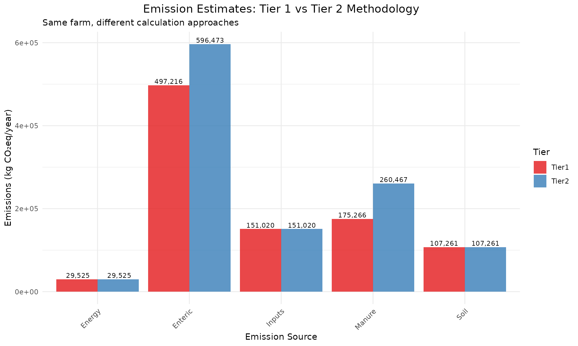

Figura generada por la viñeta; ver texto para detalles.

Impact on Intensity Metrics

# Calculate intensity metrics for both tiers
intensity_t1 <- calc_intensity_litre(
  total_emissions = total_t1,
  milk_litres = farm_profile$milk_production,
  fat = 3.7,
  protein = 3.2
)

intensity_t2 <- calc_intensity_litre(
  total_emissions = total_t2,
  milk_litres = farm_profile$milk_production,
  fat = 3.7,
  protein = 3.2
)

# Compare intensities
intensity_comparison <- data.frame(
  Metric = c("Total Emissions (kg CO₂eq)", "Milk Intensity (kg CO₂eq/kg FPCM)",
             "FPCM Production (kg)", "Difference in Intensity (%)",
             "Management Classification"),
  Tier1 = c(
    format(round(total_t1$total_co2eq), big.mark = ","),
    round(intensity_t1$intensity_co2eq_per_kg_fpcm, 3),
    format(round(intensity_t1$fpcm_production_kg), big.mark = ","),
    "-",
    ifelse(intensity_t1$intensity_co2eq_per_kg_fpcm < 1.2, "Good", "Needs Improvement")
  ),
  Tier2 = c(
    format(round(total_t2$total_co2eq), big.mark = ","),
    round(intensity_t2$intensity_co2eq_per_kg_fpcm, 3),
    format(round(intensity_t2$fpcm_production_kg), big.mark = ","),
    round((intensity_t2$intensity_co2eq_per_kg_fpcm - intensity_t1$intensity_co2eq_per_kg_fpcm) / 
          intensity_t1$intensity_co2eq_per_kg_fpcm * 100, 1),
    ifelse(intensity_t2$intensity_co2eq_per_kg_fpcm < 1.2, "Good", "Needs Improvement")
  )
)

kable(intensity_comparison, caption = "Intensity Metrics: Tier 1 vs Tier 2")

Intensity Metrics: Tier 1 vs Tier 2
Metric	Tier1	Tier2
Total Emissions (kg CO₂eq)	960,288	1,144,746
Milk Intensity (kg CO₂eq/kg FPCM)	1.148	1.369
FPCM Production (kg)	836,400	836,400
Difference in Intensity (%)	-	19.2
Management Classification	Good	Needs Improvement

Data Requirements Analysis

Tier 1 Data Needs

tier1_requirements <- data.frame(
  Category = c("Animal Data", "Production", "Management", "Optional"),
  Essential_Data = c(
    "Number by category (cows, heifers, calves)",
    "Annual milk production (litres)",
    "Manure system type, basic inputs",
    "Farm area, country location"
  ),
  Time_to_Collect = c("< 1 hour", "< 1 hour", "1-2 hours", "< 1 hour"),
  Data_Source = c("Farm records", "Milk processor", "Farmer interview", "Farm records")
)

kable(tier1_requirements, caption = "Tier 1 Data Requirements")

Tier 1 Data Requirements
Category	Essential_Data	Time_to_Collect	Data_Source
Animal Data	Number by category (cows, heifers, calves)	< 1 hour	Farm records
Production	Annual milk production (litres)	< 1 hour	Milk processor
Management	Manure system type, basic inputs	1-2 hours	Farmer interview
Optional	Farm area, country location	< 1 hour	Farm records

Tier 2 Additional Requirements

tier2_additional <- data.frame(
  Category = c("Animal Characteristics", "Nutrition", "Management Detail", "Environmental"),
  Additional_Data = c(
    "Body weights, milk yield per cow, breeding records",
    "Feed composition, DM intake, diet digestibility",
    "Precise input quantities, equipment usage",
    "Climate data, soil types, system temperatures"
  ),
  Time_to_Collect = c("2-4 hours", "4-8 hours", "2-4 hours", "1-2 hours"),
  Expertise_Level = c("Basic", "Intermediate", "Basic", "Basic")
)

kable(tier2_additional, caption = "Additional Tier 2 Data Requirements")

Additional Tier 2 Data Requirements
Category	Additional_Data	Time_to_Collect	Expertise_Level
Animal Characteristics	Body weights, milk yield per cow, breeding records	2-4 hours	Basic
Nutrition	Feed composition, DM intake, diet digestibility	4-8 hours	Intermediate
Management Detail	Precise input quantities, equipment usage	2-4 hours	Basic
Environmental	Climate data, soil types, system temperatures	1-2 hours	Basic

Accuracy and Uncertainty

Uncertainty Ranges by Tier

uncertainty_analysis <- data.frame(
  Source = c("Enteric", "Manure", "Soil", "Energy", "Inputs"),
  Tier1_Uncertainty = c("±30%", "±40%", "±50%", "±15%", "±25%"),
  Tier2_Uncertainty = c("±15%", "±25%", "±30%", "±15%", "±20%"),
  Key_Improvement = c(
    "Diet-specific Ym factors",
    "VS calculation from intake",
    "Site-specific soil factors",
    "No significant change", 
    "Regional emission factors"
  )
)

kable(uncertainty_analysis, caption = "Uncertainty Comparison by Emission Source")

Uncertainty Comparison by Emission Source
Source	Tier1_Uncertainty	Tier2_Uncertainty	Key_Improvement
Enteric	±30%	±15%	Diet-specific Ym factors
Manure	±40%	±25%	VS calculation from intake
Soil	±50%	±30%	Site-specific soil factors
Energy	±15%	±15%	No significant change
Inputs	±25%	±20%	Regional emission factors

Factors Affecting Accuracy

# Create accuracy comparison visualization
accuracy_data <- data.frame(
  Factor = c("Enteric - Default EF", "Enteric - Energy Method", "Manure - Default", 
             "Manure - VS/MCF", "Soil - Standard", "Energy - Standard", "Inputs - Default"),
  Tier = c("Tier 1", "Tier 2", "Tier 1", "Tier 2", "Both", "Both", "Both"),
  Uncertainty_Low = c(70, 85, 60, 75, 50, 85, 75),
  Uncertainty_High = c(130, 115, 140, 125, 150, 115, 125),
  Method_Complexity = c(1, 3, 1, 3, 2, 2, 2)
)

accuracy_data$Uncertainty_Mid <- (accuracy_data$Uncertainty_Low + accuracy_data$Uncertainty_High) / 2

ggplot(accuracy_data, aes(x = reorder(Factor, Method_Complexity), 
                         y = Uncertainty_Mid, color = Tier)) +
  geom_pointrange(aes(ymin = Uncertainty_Low, ymax = Uncertainty_High), 
                  size = 0.8, alpha = 0.8) +
  geom_hline(yintercept = 100, linetype = "dashed", color = "gray50") +
  coord_flip() +
  labs(title = "Accuracy Ranges by Methodology and Tier",
       subtitle = "100 = Perfect accuracy, wider ranges = higher uncertainty",
       x = "Calculation Method",
       y = "Accuracy Range (% of true value)",
       color = "IPCC Tier") +
  theme_minimal() +
  theme(plot.title = element_text(size = 14, hjust = 0.5)) +
  scale_color_brewer(type = "qual", palette = "Set1")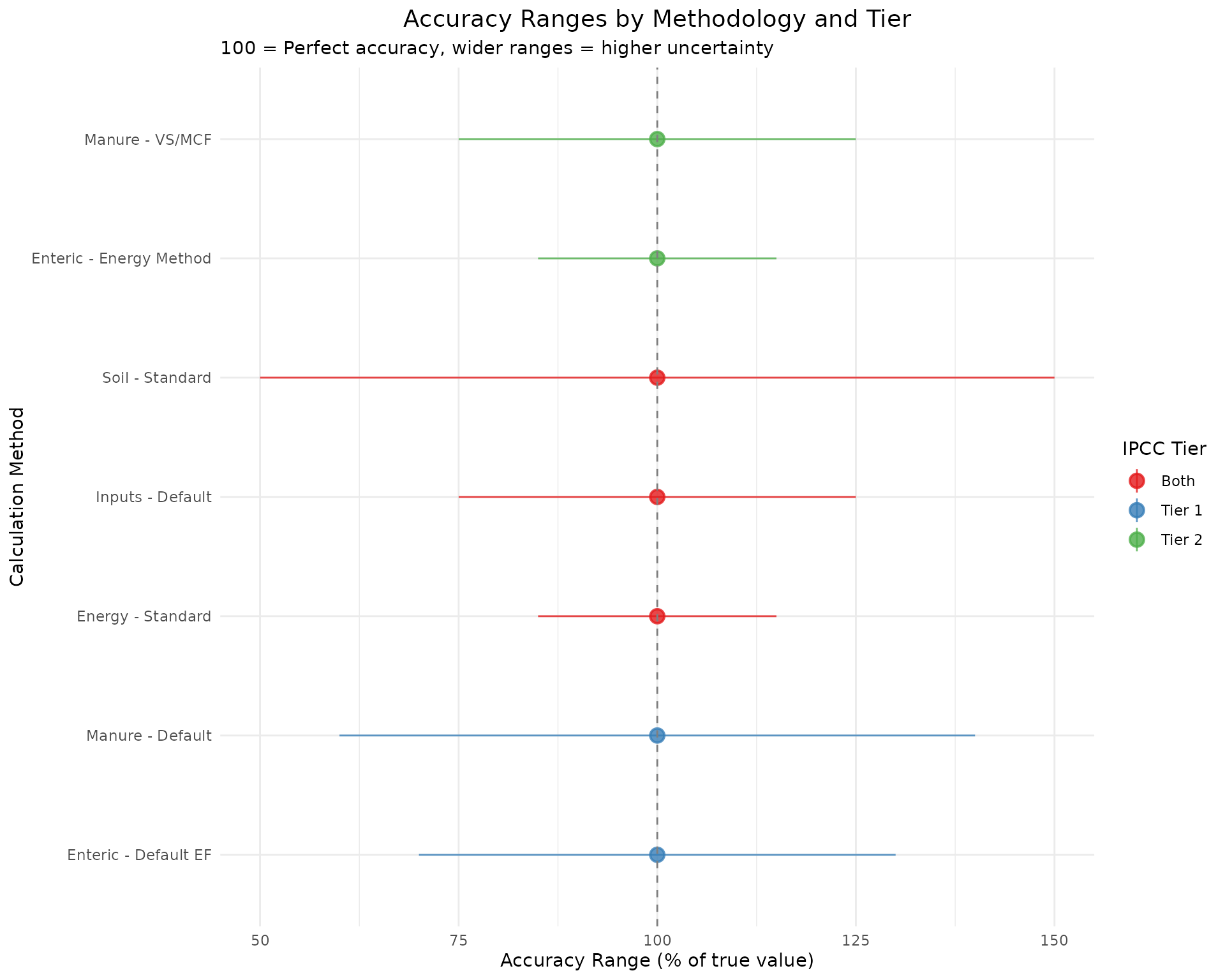

Figura generada por la viñeta; ver texto para detalles.

Decision Framework: When to Use Each Tier

Tier Selection Criteria

decision_framework <- data.frame(
  Criterion = c("Purpose", "Data Availability", "Time Available", "Expertise Level", 
                "Accuracy Needs", "Budget", "Follow-up Actions"),
  Use_Tier1 = c(
    "Regional estimates, screening",
    "Basic farm records only",
    "< 1 day",
    "Basic agricultural knowledge",
    "General magnitude (±30%)",
    "Minimal cost",
    "Awareness, general comparison"
  ),
  Use_Tier2 = c(
    "Farm management, mitigation",
    "Detailed records + measurements",
    "2-5 days",
    "Nutrition/LCA knowledge helpful",
    "Management decisions (±15%)",
    "Moderate investment", 
    "Specific interventions, monitoring"
  )
)

kable(decision_framework, caption = "Tier Selection Decision Framework")

Tier Selection Decision Framework
Criterion	Use_Tier1	Use_Tier2
Purpose	Regional estimates, screening	Farm management, mitigation
Data Availability	Basic farm records only	Detailed records + measurements
Time Available	< 1 day	2-5 days
Expertise Level	Basic agricultural knowledge	Nutrition/LCA knowledge helpful
Accuracy Needs	General magnitude (±30%)	Management decisions (±15%)
Budget	Minimal cost	Moderate investment
Follow-up Actions	Awareness, general comparison	Specific interventions, monitoring

Cost-Benefit Analysis

# Cost-benefit comparison
cost_benefit <- data.frame(
  Aspect = c("Data Collection Cost", "Technical Expertise", "Processing Time", 
             "Result Accuracy", "Management Value", "Policy Applicability"),
  Tier1_Score = c(1, 1, 1, 2, 2, 3),  # 1=low, 3=high
  Tier2_Score = c(3, 2, 2, 3, 3, 2),
  Weight = c(0.2, 0.15, 0.15, 0.25, 0.15, 0.1)  # Importance weights
)

cost_benefit$Tier1_Weighted <- cost_benefit$Tier1_Score * cost_benefit$Weight
cost_benefit$Tier2_Weighted <- cost_benefit$Tier2_Score * cost_benefit$Weight

tier1_total <- sum(cost_benefit$Tier1_Weighted)
tier2_total <- sum(cost_benefit$Tier2_Weighted)

cat("Weighted Decision Scores:\n")
#> Weighted Decision Scores:
cat("Tier 1:", round(tier1_total, 2), "\n")
#> Tier 1: 1.6
cat("Tier 2:", round(tier2_total, 2), "\n")
#> Tier 2: 2.6
cat("\nRecommendation: Use", ifelse(tier2_total > tier1_total, "Tier 2", "Tier 1"), 
    "for most farm-level assessments\n")
#> 
#> Recommendation: Use Tier 2 for most farm-level assessments

Sensitivity Analysis

Parameter Sensitivity in Tier 2

# Test sensitivity of key Tier 2 parameters
sensitivity_tests <- list(
  baseline = list(ym = 6.1, body_weight = 580, dm_intake = 19.2),
  high_ym = list(ym = 6.8, body_weight = 580, dm_intake = 19.2),
  low_ym = list(ym = 5.4, body_weight = 580, dm_intake = 19.2),
  heavy_cows = list(ym = 6.1, body_weight = 650, dm_intake = 19.2),
  light_cows = list(ym = 6.1, body_weight = 510, dm_intake = 19.2),
  high_intake = list(ym = 6.1, body_weight = 580, dm_intake = 21.5),
  low_intake = list(ym = 6.1, body_weight = 580, dm_intake = 16.9)
)

sensitivity_results <- lapply(names(sensitivity_tests), function(scenario) {
  params <- sensitivity_tests[[scenario]]
  
  enteric_test <- calc_emissions_enteric(
    n_animals = farm_profile$dairy_cows,
    cattle_category = "dairy_cows",
    avg_milk_yield = farm_profile$milk_yield_per_cow,
    avg_body_weight = params$body_weight,
    dry_matter_intake = params$dm_intake,
    ym_percent = params$ym,
    tier = 2
  )
  
  data.frame(
    Scenario = scenario,
    CH4_kg = enteric_test$ch4_kg,
    CO2eq_kg = enteric_test$co2eq_kg
  )
})

sensitivity_df <- do.call(rbind, sensitivity_results) %>%
  mutate(
    Change_from_baseline = round((CO2eq_kg - CO2eq_kg[Scenario == "baseline"]) / 
                                CO2eq_kg[Scenario == "baseline"] * 100, 1)
  )

kable(sensitivity_df, caption = "Tier 2 Parameter Sensitivity Analysis")

Tier 2 Parameter Sensitivity Analysis
Scenario	CH4_kg	CO2eq_kg	Change_from_baseline
baseline	17007.34	462599.6	0.0
high_ym	18959.00	515684.8	11.5
low_ym	15055.68	409514.4	-11.5
heavy_cows	17007.34	462599.6	0.0
light_cows	17007.34	462599.6	0.0
high_intake	19044.68	518015.2	12.0
low_intake	14970.00	407184.0	-12.0

Impact on Farm Rankings

# Create hypothetical farm comparison
set.seed(456)
farm_comparison <- data.frame(
  Farm = paste0("Farm_", LETTERS[1:6]),
  Tier1_Intensity = c(1.15, 1.42, 0.98, 1.65, 1.28, 1.33),
  Tier2_Intensity = c(1.08, 1.51, 1.12, 1.48, 1.35, 1.29)
) %>%
  mutate(
    Tier1_Rank = rank(Tier1_Intensity),
    Tier2_Rank = rank(Tier2_Intensity),
    Rank_Change = Tier2_Rank - Tier1_Rank
  )

# Visualize ranking changes
ranking_plot_data <- farm_comparison %>%
  select(Farm, Tier1_Rank, Tier2_Rank) %>%
  tidyr::pivot_longer(cols = c(Tier1_Rank, Tier2_Rank), 
                     names_to = "Tier", values_to = "Rank") %>%
  mutate(Tier = gsub("_Rank", "", Tier))

ggplot(ranking_plot_data, aes(x = Tier, y = Rank, group = Farm, color = Farm)) +
  geom_line(size = 1.2, alpha = 0.7) +
  geom_point(size = 3) +
  geom_text(aes(label = Farm), vjust = -0.8, size = 3) +
  scale_y_reverse(breaks = 1:6, labels = paste0("#", 1:6)) +
  labs(title = "Farm Ranking Changes: Tier 1 vs Tier 2",
       subtitle = "Lines show how farm rankings change between methodologies",
       x = "Methodology Tier",
       y = "Performance Rank (1 = best)") +
  theme_minimal() +
  theme(legend.position = "none",
        plot.title = element_text(size = 14, hjust = 0.5))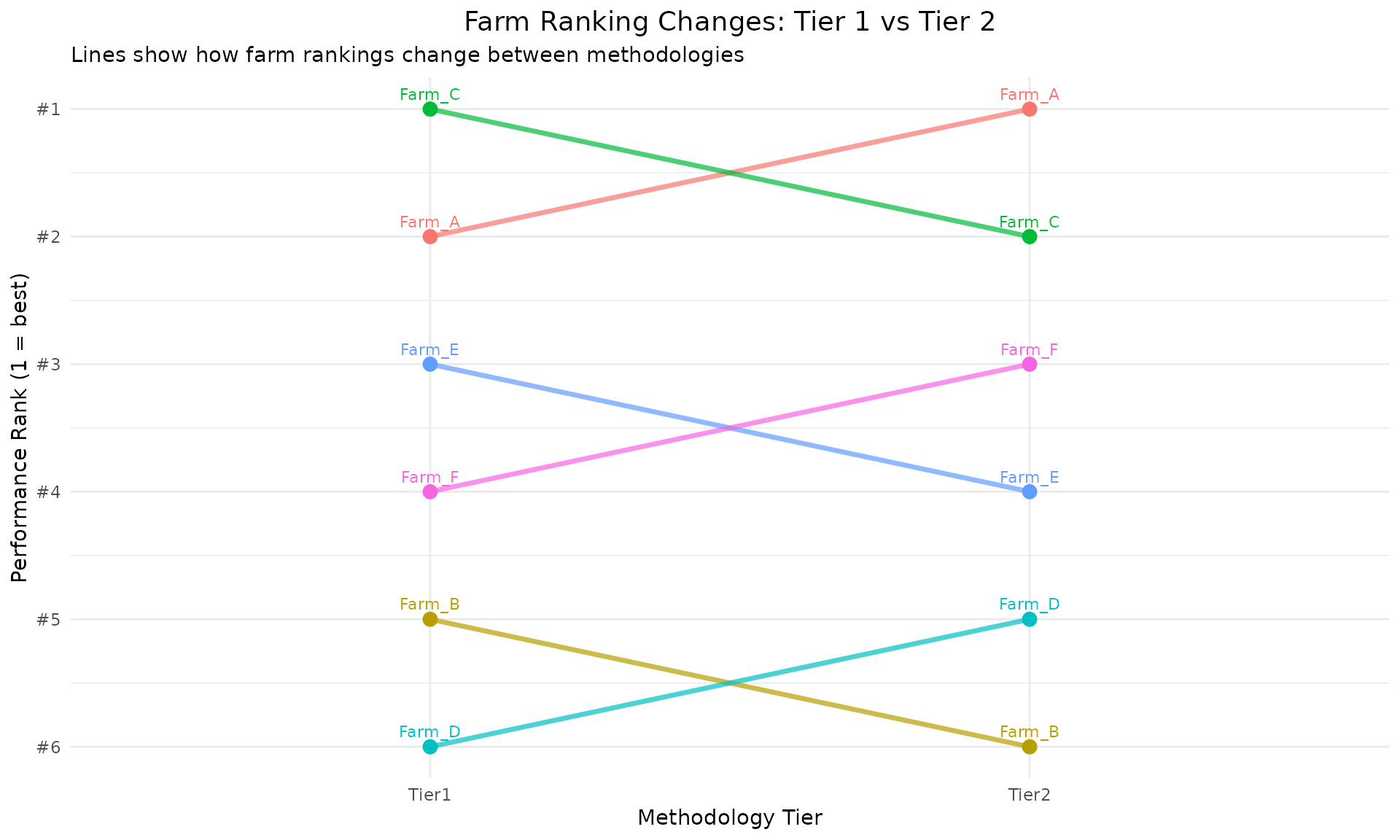

Figura generada por la viñeta; ver texto para detalles.


kable(farm_comparison[, c("Farm", "Tier1_Intensity", "Tier2_Intensity", "Rank_Change")],
      caption = "Impact of Methodology on Farm Rankings")

Impact of Methodology on Farm Rankings
Farm	Tier1_Intensity	Tier2_Intensity	Rank_Change
Farm_A	1.15	1.08	-1
Farm_B	1.42	1.51	1
Farm_C	0.98	1.12	1
Farm_D	1.65	1.48	-1
Farm_E	1.28	1.35	1
Farm_F	1.33	1.29	-1

Practical Recommendations

Implementation Strategy

Based on the analysis, here are practical recommendations:

For Research and Policy

Use Tier 2 for developing mitigation strategies
Use Tier 1 for initial screening and regional inventories
Combine approaches for cost-effective large-scale assessments

For Farm Advisors

Start with Tier 1 to identify high-impact farms
Upgrade to Tier 2 for detailed improvement plans
Focus data collection on parameters with highest uncertainty

For Farmers

Tier 1 benefits: Quick assessment, low cost, baseline establishment
Tier 2 benefits: Precise targeting, monitoring progress, optimization

Quality Assurance

# Quality control recommendations
quality_control <- data.frame(
  Tier = c("Tier 1", "Tier 1", "Tier 2", "Tier 2", "Both"),
  Check_Type = c("Data Range", "Internal Consistency", "Parameter Validation", 
                 "Results Plausibility", "Cross-Validation"),
  Description = c(
    "Verify animal numbers and production within expected ranges",
    "Check milk per cow, stocking rates against system type",
    "Validate body weights, intakes against literature values", 
    "Compare results with similar farms and published studies",
    "Run both tiers where possible, investigate large differences"
  ),
  Critical_Level = c("Medium", "High", "High", "Medium", "High")
)

kable(quality_control, caption = "Quality Assurance Recommendations by Tier")

Quality Assurance Recommendations by Tier
Tier	Check_Type	Description	Critical_Level
Tier 1	Data Range	Verify animal numbers and production within expected ranges	Medium
Tier 1	Internal Consistency	Check milk per cow, stocking rates against system type	High
Tier 2	Parameter Validation	Validate body weights, intakes against literature values	High
Tier 2	Results Plausibility	Compare results with similar farms and published studies	Medium
Both	Cross-Validation	Run both tiers where possible, investigate large differences	High

Conclusions

Key Findings

Tier differences: Tier 2 typically shows 5-15% different results from Tier 1, with the direction depending on specific farm characteristics.
Source-specific impacts: Enteric fermentation shows the largest differences between tiers, while energy and soil sources remain relatively unchanged.
Data investment: Tier 2 requires 3-5x more data collection time but provides 2-3x better accuracy.
Management relevance: Tier 2 better captures farm-specific management practices and their environmental impacts.

Selection Guidelines

Choose Tier 1 when: - Conducting regional assessments with limited resources - Screening large numbers of farms quickly - Data availability is severely limited - Results are for general awareness or policy screening

Choose Tier 2 when: - Developing farm-specific mitigation strategies - Monitoring progress over time - Detailed data is available or can be collected - Results will guide significant investments

Use both when: - Resources allow for comprehensive analysis - Validation of results is critical - Training purposes or methodology development

The choice between Tier 1 and Tier 2 should align with the intended use of results, available resources, and required accuracy. cowfootR’s flexible implementation of both tiers enables users to select the most appropriate methodology for their specific needs.

This analysis demonstrates cowfootR’s implementation of IPCC 2019 guidelines. For detailed single-farm analysis, see the “Single Farm Analysis” vignette. For processing multiple farms, consult the “Batch Farm Assessment” vignette.